I realized that for my final finding to make sense I would need to share some more relevant data. Firstly I have confirmed Evans finding that blue and green inserters have a spin time of 24 ticks. This doesn't really make sense as red inserters are 50 ticks, and these inserters are exactly twice as fast, meaning we should be getting 25 ticks, yet the number is 24 despite that. Once again this is a discrepancy that has no real explanation.
Anyway doing all the same calculations as before we find a cost per motion of ~47.957kw, a cost per spin of ~23.1844kJ, and an operating cost of ~58.961kw. This is once again quite similar to Evans empirical data, but very different to the games hard coded data. It also makes me question if I misinterpreted the data when looking at the yellow inserter since the games hardcoded value is 5kj, I assumed this meant it would use 5kw when moving, but now looking at the green inserter as reference that actually seems to be kJ per full spin, not kw cost of motion as I originally interpreted. In that case me and the game actually have a discrepancy of ~1.6kJ on the yellow inserter, and our discrepancy on the green inserter is twice as high. This unfortunately means we can't actually trust the game, as it seems to just be lying about everything at every turn. Even something as basic as the inserters spin speed. Sure the yellow and burner inserter had a rounding error so we can understand, but the green and blue inserters should be doing exactly 25 ticks per spin. Its perfect math, and yet they do 24.
At this point my attempts to walk away have been foiled as I am completely baffled by this. I was ready to just use the in game data to make some calculations assuming they'd be accurate as long as tick rounding wasn't introduced, but for no reason at all that doesn't work. Those devs are cheeky liars, and now I've been sucked right back in. Interestingly our numbers for the red inserter seem to be basically perfect with what the game tells us, its just all these short ones that make no sense.
Anyway since I'm already here I'll just do the blue inserters. Originally I was going to neglect them since they should obviously just be worse in every use case, but given the game has lied about everything else so far we need to confirm this as well. Once again I confirmed 24 ticks rotation (so thankfully that is consistent at least). We get a cost of motion of ~16.7414 kw, a cost per spin of ~8.1151kJ. Interestingly, though this is still objectively the worst inserter in terms of kJ per item, the disparity is not as huge as the game leads you to believe. ~6.6kJ for the yellow inserter, almost a perfect 7kJ for the red, and for the blue just ~8.1kJ. Anyway this gives us an operating cost of ~20.7879kW.
For the burner inserter, I still haven't collected better data than before, so this number won't be as accurate as it could be, but just so we have something for reference for current comparison I'll finish the calculation with the data from last time. I'll be using the operating cost from coal as the reference, as I am most interested in their practicality fueling boilers with coal in the early game. Obviously solid fuel is three times denser, so if they can do coal they can do solid fuel easily. If you are interested in the solid fuel use case you are welcome to do the calculation as all the data is present. the ~53.8kw operating cost from coal can be reverse engineered into our previous equations, giving us a cost per spin of ~68.1466kJ. For completeness I will also derive the cost of motion, though we don't actually need it for anything at this point, and that value is ~51.36216kW.
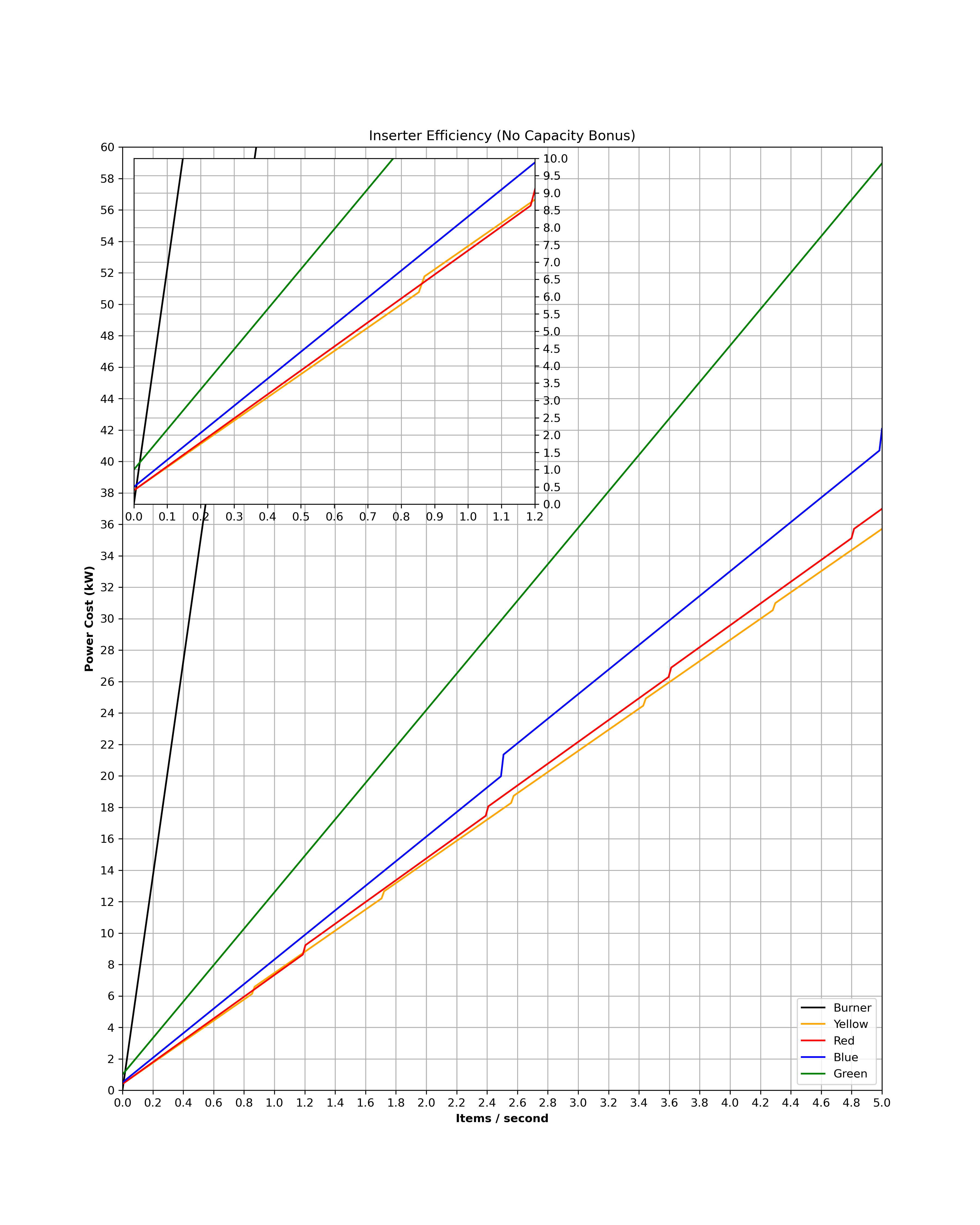
Now lets derive the actual interpretation of this data. Which inserter should be used at how many item/s. I went ahead and whipped up some graphs in python because I'm cool like that

- download.png (612.59 KiB) Viewed 5658 times
Source code for the graph
Code: Select all
import matplotlib.pyplot as plt
import numpy as np
from mpl_toolkits.axes_grid1.inset_locator import zoomed_inset_axes

stack_size = 1
green_stack = 2

yellow_speed = 60 / 70
red_speed = 60 / 50
blue_speed = 60 / 24

burner_energy = 68.1466
yellow_energy = 6.65203
red_energy = 7
blue_energy = 8.1151
green_energy = 23.1844

yellow_drain = 0.4
blue_drain = 0.5
green_drain = 1

x = np.linspace(0, 2.5 * green_stack, 300)

yellow_mod = x % (yellow_speed * stack_size)
red_mod = x % (red_speed * stack_size)
blue_mod = x % (blue_speed * stack_size)

burner = (burner_energy / stack_size) * x
yellow = ((yellow_energy / stack_size) * x) + (yellow_drain * (((x / yellow_speed) - yellow_mod) + 1))
red = ((red_energy / stack_size) * x) + (yellow_drain * (((x / red_speed) - red_mod) + 1))
blue = ((blue_energy / stack_size) * x) + (blue_drain * (((x / blue_speed) - blue_mod) + 1))
green = ((green_energy / green_stack) * x) + green_drain

fig = plt.figure(figsize = (12, 15), dpi = 300)
ax = plt.axes()

ax.plot(x, burner, label = "Burner", color = "black")
ax.plot(x, yellow, label = "Yellow", color = "orange")
ax.plot(x, red, label = "Red", color = "red")
ax.plot(x, blue, label = "Blue", color = "blue")
ax.plot(x, green, label = "Green", color = "green")

ylim = 60

ax.set_ylim(0, ylim)
ax.set_xlim(0, blue_speed * green_stack)

xtick = 0.2 * green_stack
ytick = 2

ax.set_xticks(np.arange(0, blue_speed * green_stack + xtick, xtick))
ax.set_yticks(np.arange(0, ylim + ytick, ytick))

ax.set_title("Inserter Efficiency (No Capacity Bonus)")
ax.set_xlabel("Items / second", fontweight = "bold")
ax.set_ylabel("Power Cost (kW)", fontweight = "bold")

ax.grid()
ax.legend(loc = 4)

zax = zoomed_inset_axes(ax, 2.2, loc = 2, borderpad = 1)
zax.yaxis.tick_right()

zax.plot(x, burner, label = "Burner", color = "black")
zax.plot(x, yellow, label = "Yellow", color = "orange")
zax.plot(x, red, label = "Red", color = "red")
zax.plot(x, blue, label = "Blue", color = "blue")
zax.plot(x, green, label = "Green", color = "green")


zylim = 10
zxlim = red_speed * stack_size

zax.set_ylim(0, zylim)
zax.set_xlim(0, zxlim)

zxtick = 0.1 * green_stack
zytick = 0.5

zax.set_xticks(np.arange(0, zxlim + zxtick, zxtick))
zax.set_yticks(np.arange(0, zylim + zytick, zytick))

zax.grid()

plt.show()
So here are our default values. As you can see burners shoot off into the sun so we practically can't make out what they're doing at all. I added a zoom in to help clarify some things in the initial corner. The graph is setup so that when an inserter reaches its maximum capacity, it will be assumed a second inserter is being used in tandem to continue increasing throughput. This is why the graph has those bumps, as a second inserter worth of drain is added.
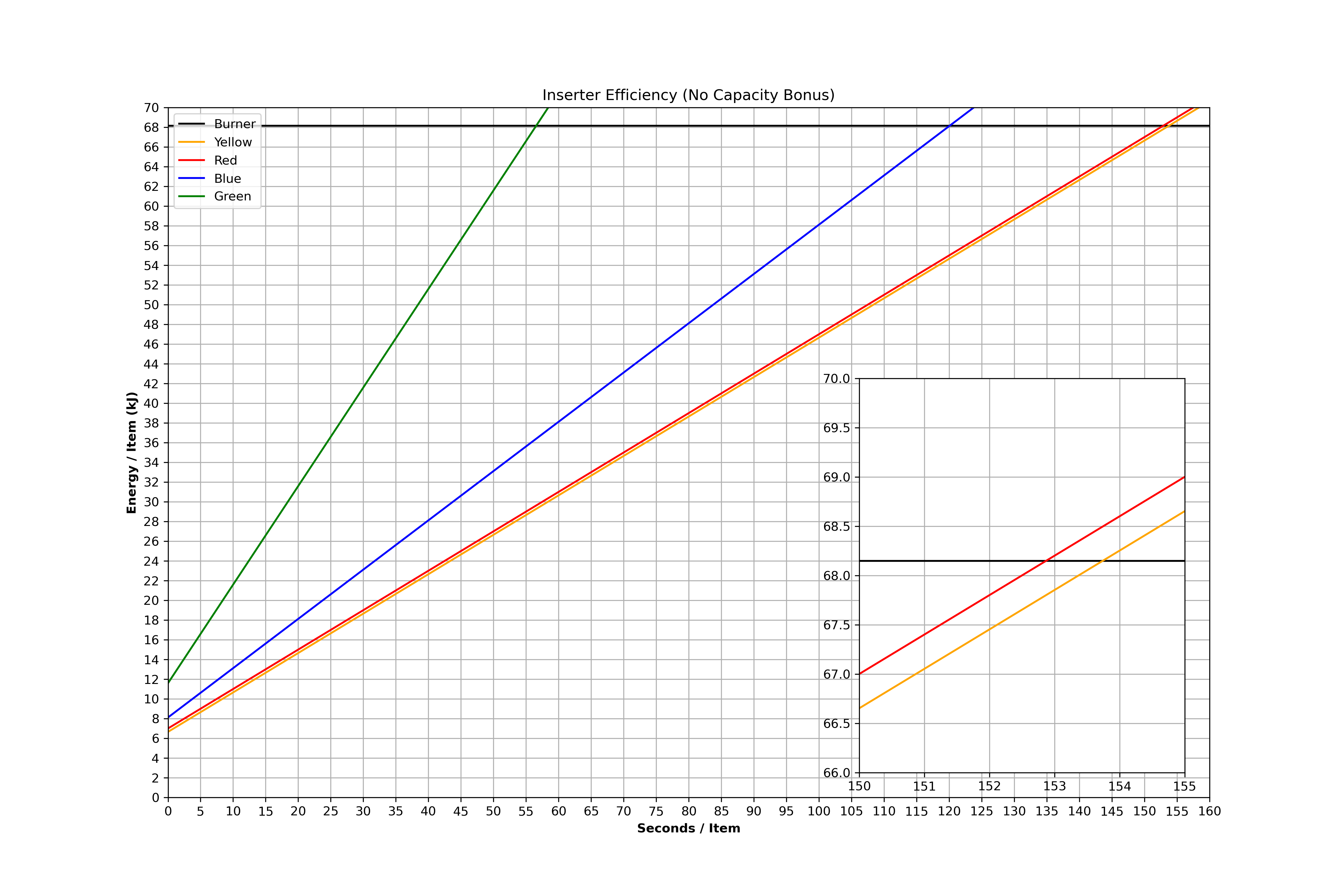
Now we can continue generating quite a few variations of these graphs at various stack sizes. I've decided its a bit impractical to just bombard people with literally dozens of graphs, so we'll just focus on some key ones. First we will show at what point burners become more profitable than yellow inserters. To do this we will just inverse the x axis on our graph by flipping our speed values, and a little finagling with the code so it looks right, and we get this:
- download2 (2).png (472.5 KiB) Viewed 5658 times
Code: Select all
import matplotlib.pyplot as plt
import numpy as np
from mpl_toolkits.axes_grid1.inset_locator import zoomed_inset_axes

stack_size = 1
green_stack = 2


yellow_speed = 70 / 60
red_speed = 50 / 60
blue_speed = 24 / 60

burner_energy = 68.1466
yellow_energy = 6.65203
red_energy = 7
blue_energy = 8.1151
green_energy = 23.1844

yellow_drain = 0.4
blue_drain = 0.5
green_drain = 1

x = np.linspace(0, 300, 300)

yellow_mod = x % (yellow_speed * stack_size)
red_mod = x % (red_speed * stack_size)
blue_mod = x % (blue_speed * stack_size)

burner = (burner_energy / stack_size)
yellow = (yellow_energy / stack_size) + (yellow_drain * x)
red = (red_energy / stack_size) + (yellow_drain * x)
blue = (blue_energy / stack_size) + (blue_drain * x)
green = (green_energy / green_stack) + (green_drain * x)

fig = plt.figure(figsize = (15, 10), dpi = 300)
ax = plt.axes()

plt.axhline(y = burner, label = "Burner", color = "black")
ax.plot(x, yellow, label = "Yellow", color = "orange")
ax.plot(x, red, label = "Red", color = "red")
ax.plot(x, blue, label = "Blue", color = "blue")
ax.plot(x, green, label = "Green", color = "green")

ylim = 70
xlim = 160

ax.set_ylim(0, ylim)
ax.set_xlim(0, xlim)

xtick = 5
ytick = 2

ax.set_xticks(np.arange(0, xlim + xtick, xtick))
ax.set_yticks(np.arange(0, ylim + ytick, ytick))

ax.set_title("Inserter Efficiency (No Capacity Bonus)")
ax.set_xlabel("Seconds / Item", fontweight = "bold")
ax.set_ylabel("Energy / Item (kJ)", fontweight = "bold")

ax.grid()
ax.legend(loc = 4)

plt.show()
This data is pretty self explanatory, and I've zoomed in on points of interests. As we can see there is a point where a red inserter does become more efficient than a yellow one, and that is when a single yellow inserter is maxed so you'd need a second one, but the single red inserter still has some breathing room. As for the burner, we find that it becomes the best inserter when moving less than 1 item every ~2.5 minutes. Remember all inserters are subject to the same ratio since they share a stack size, except for green inserters. But the green inserter never makes a dent in that graph regardless of its stack size advantage, so there's no point in looking further. Just divide the time by the stack size to account the upgraded time. Also remember our numbers for the burner might not be perfectly accurate.
- download3.png (601.46 KiB) Viewed 5658 times
Code: Select all
import matplotlib.pyplot as plt
import numpy as np
from mpl_toolkits.axes_grid1.inset_locator import zoomed_inset_axes

stack_size = 2
green_stack = 6

yellow_speed = 60 / 70
red_speed = 60 / 50
blue_speed = 60 / 24

burner_energy = 68.1466
yellow_energy = 6.65203
red_energy = 7
blue_energy = 8.1151
green_energy = 23.1844

yellow_drain = 0.4
blue_drain = 0.5
green_drain = 1

x = np.linspace(0, blue_speed * green_stack, 300)

yellow_mod = x % (yellow_speed * stack_size)
red_mod = x % (red_speed * stack_size)
blue_mod = x % (blue_speed * stack_size)

burner = (burner_energy / stack_size) * x
yellow = ((yellow_energy / stack_size) * x) + (yellow_drain * (((x / yellow_speed) - yellow_mod) + 1))
red = ((red_energy / stack_size) * x) + (yellow_drain * (((x / red_speed) - red_mod) + 1))
blue = ((blue_energy / stack_size) * x) + (blue_drain * (((x / blue_speed) - blue_mod) + 1))
green = ((green_energy / green_stack) * x) + green_drain

fig = plt.figure(figsize = (12, 15), dpi = 300)
ax = plt.axes()

ax.plot(x, burner, label = "Burner", color = "black")
ax.plot(x, yellow, label = "Yellow", color = "orange")
ax.plot(x, red, label = "Red", color = "red")
ax.plot(x, blue, label = "Blue", color = "blue")
ax.plot(x, green, label = "Green", color = "green")

ylim = 60
xlim = blue_speed * green_stack

ax.set_ylim(0, ylim)
ax.set_xlim(0, xlim)

xtick = 0.6
ytick = 2

ax.set_xticks(np.arange(0, xlim + xtick, xtick))
ax.set_yticks(np.arange(0, ylim + ytick, ytick))

ax.set_title("Inserter Efficiency (Capacity Bonus 4)")
ax.set_xlabel("Items / second", fontweight = "bold")
ax.set_ylabel("Power Cost (kW)", fontweight = "bold")

ax.grid()
ax.legend(loc = 4)

zax = zoomed_inset_axes(ax, 3, loc = 2, borderpad = 1)
zax.yaxis.tick_right()

zax.plot(x, burner, label = "Burner", color = "black")
zax.plot(x, yellow, label = "Yellow", color = "orange")
zax.plot(x, red, label = "Red", color = "red")
zax.plot(x, blue, label = "Blue", color = "blue")
zax.plot(x, green, label = "Green", color = "green")


zylim = 10
zxlim = red_speed * stack_size

zax.set_ylim(16, 24)
zax.set_xlim(4.2, 5.4)

zxtick = 0.2
zytick = 0.5

zax.set_xticks(np.arange(4.2, 5.4 + zxtick, zxtick))
zax.set_yticks(np.arange(16, 24 + zytick, zytick))

zax.grid()

plt.show()
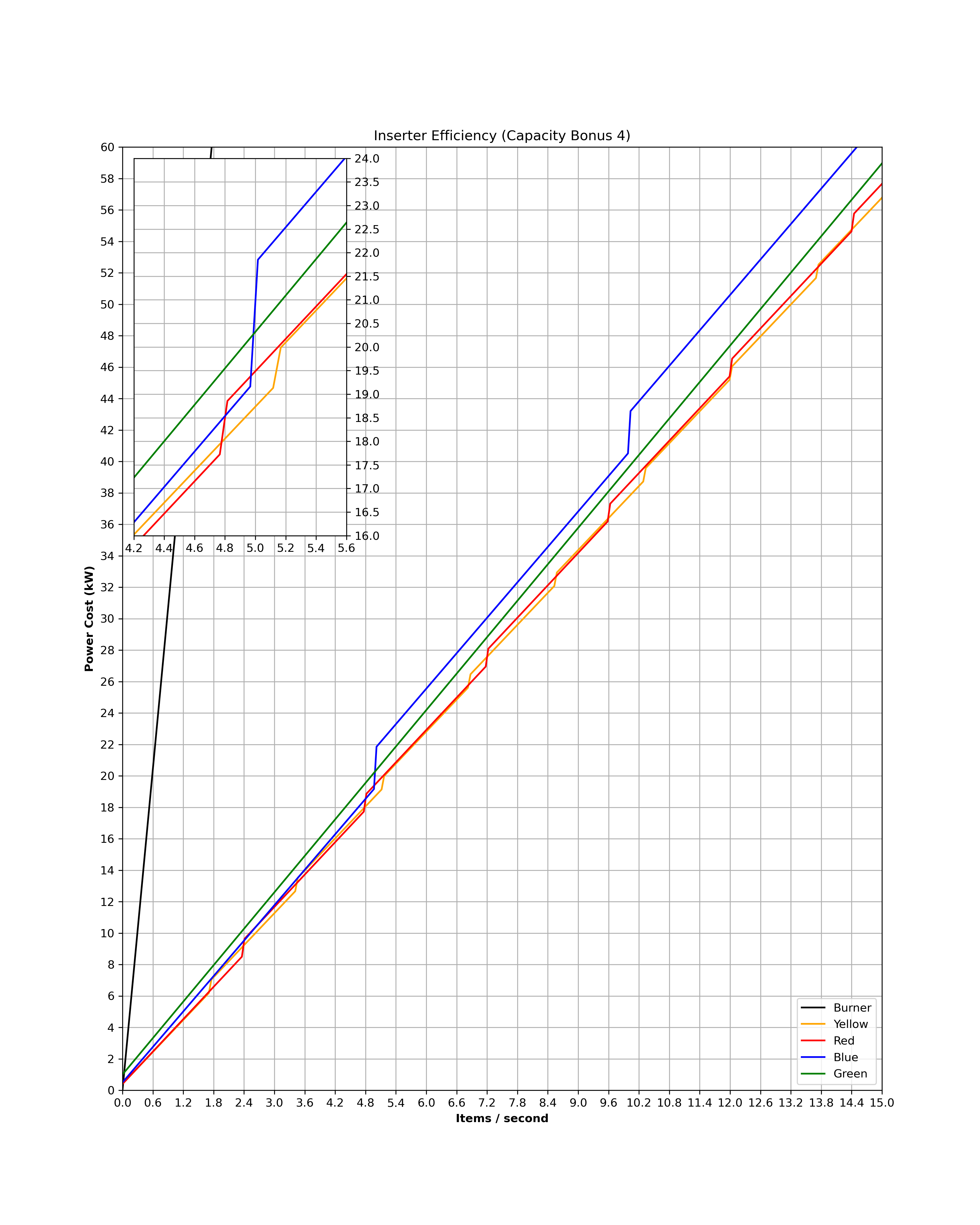
Now this is is a very interesting graph. Remember that between Capacity Bonus 2 and Capacity Bonus 7, the only inserter affected is the green one, and all the others remain the same at a a stack size of 2. The graph actually tells us a couple different things. Firstly, at capacity bonus 2 we can see that the red and yellow inserter now regularly exchange in a kind of interlaced pattern. That means for anyone trying to optimize efficiency it actually is important to reference the graph and maybe do the calculation. Very cool! We can also that the blue inserter is always more expensive if not equally expensive to the other inserters, except for a brief point around 4.9 items per second where it does actually become cheaper than red inserters. I think this range is too small to have any practical significance, but its noteworthy. We can also see that at a throughput of 5 items per second or higher, green inserters begin destroying blue inserters. This is the first time a green inserter overtakes one of the other inserters in the game, which is why I chose capacity bonus 4 for this graph.
- download4.png (581.47 KiB) Viewed 5658 times
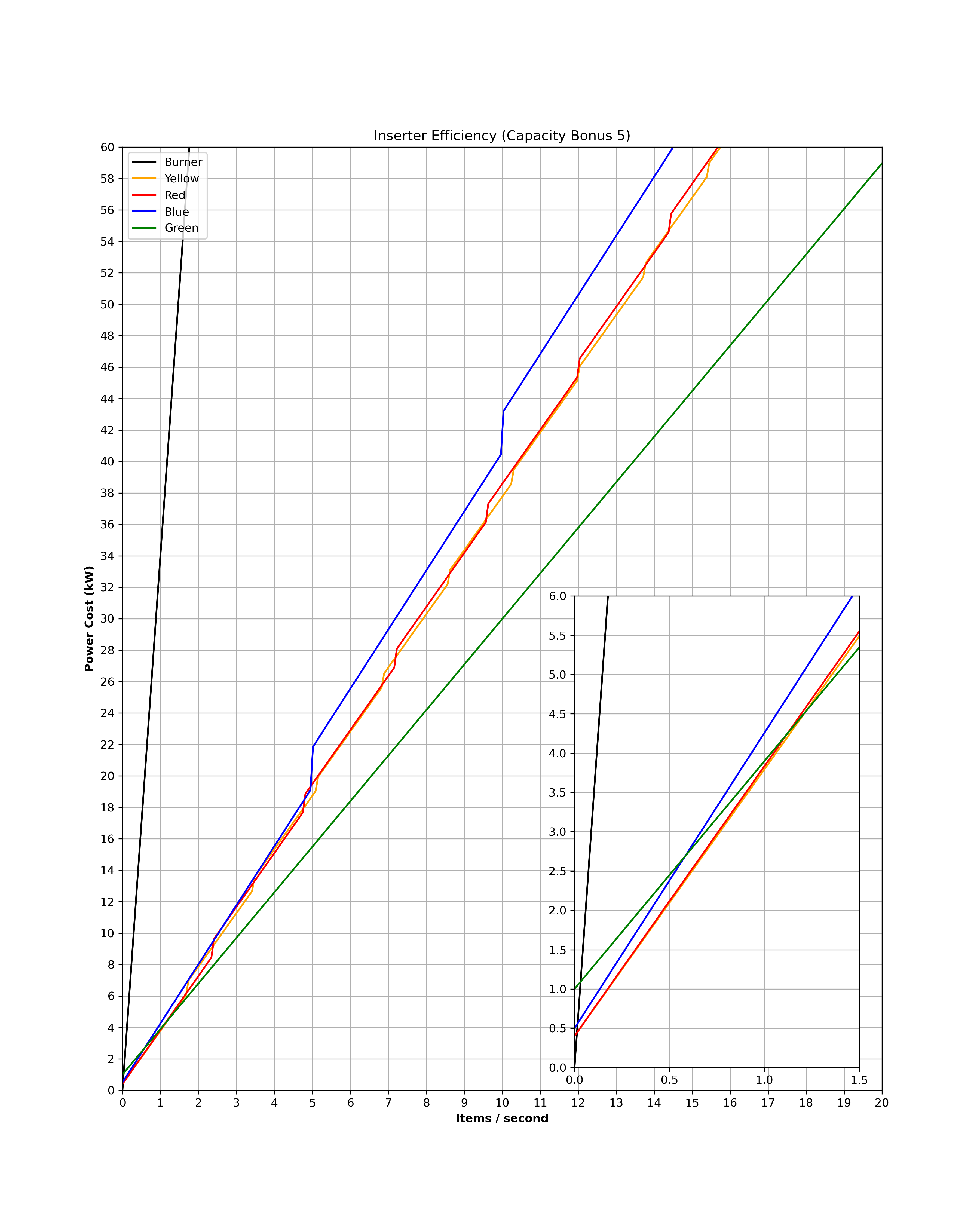
Here we can see Green Inserters start dominating. The other inserters only remain viable in the lower throughputs. Granted there are still many use cases with a throughput that low, but it really doesn't take very much at all for the green inserter to pull ahead stupendously. We can also see that by this point the blue inserter has become completely obsolete. At capacity 4 it will still barely holding onto relevance, but now its just completely smoked. Here is the green inserter being even more dominant:
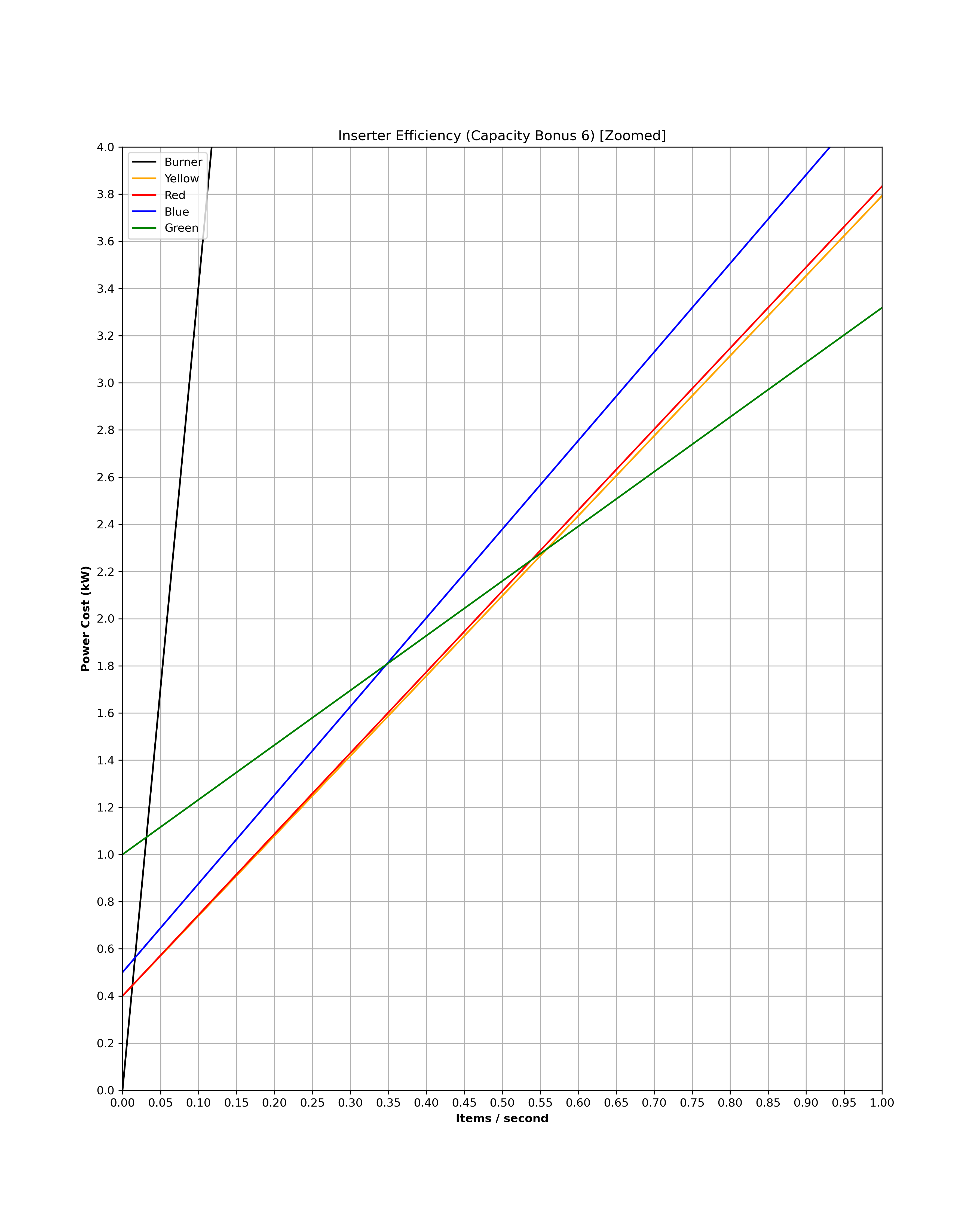
- download5.png (445.46 KiB) Viewed 5658 times
Finally the coup de grace, Capacity Bonus 7:
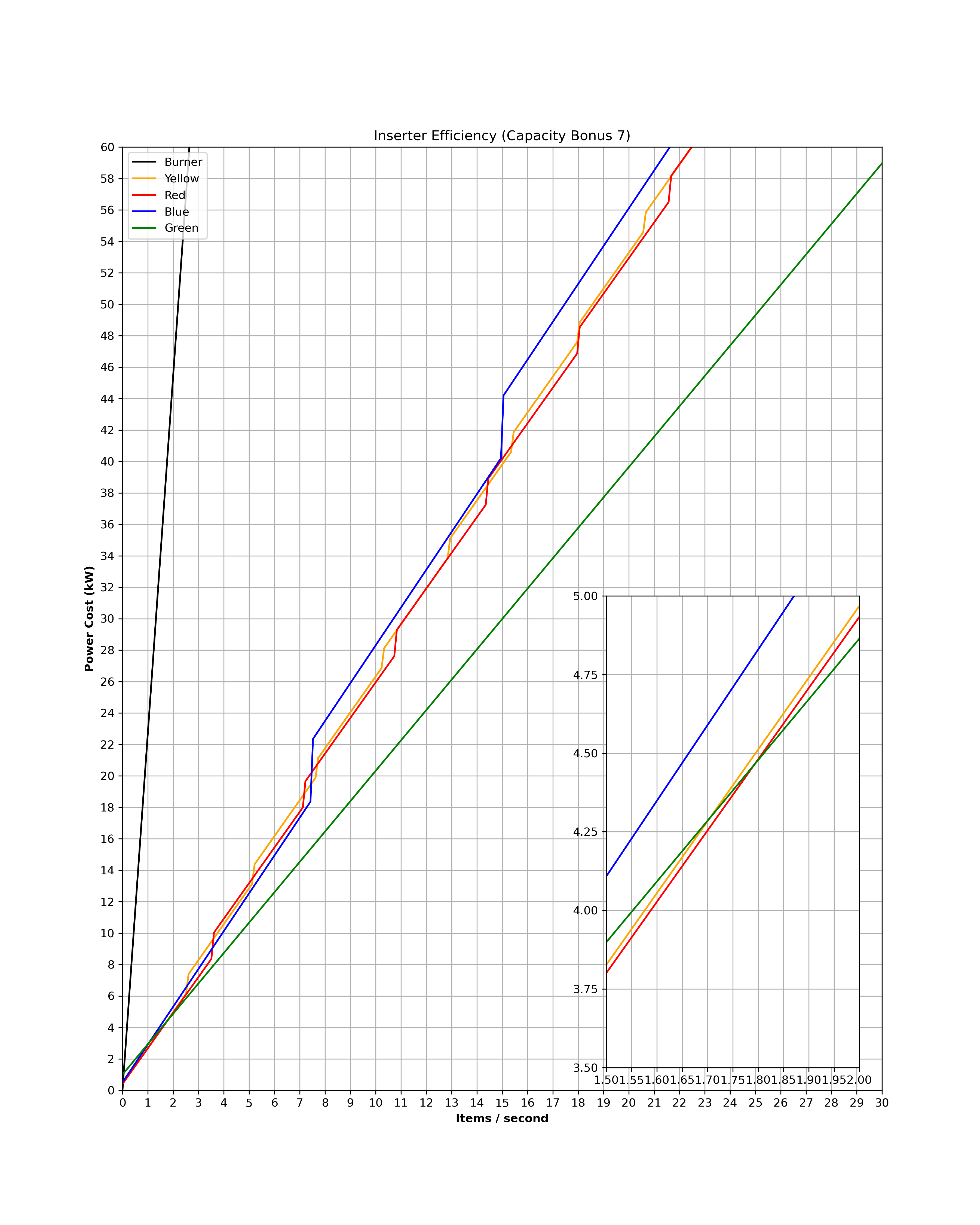
- download6.png (573.84 KiB) Viewed 5658 times
Here we can see the blue inserter regain a little bit of relevance over its counterparts, but the green inserters still blow all of them away. We can see from the zoom in this occurs around a throughput of 1.5 items/s, and before that the red and yellow inserters dominate. Also interestingly on our zoom in we see that red inserters have somehow overtaken yellow inserters? I'm not really sure how that's possible as their relationship should be proportional between stack sizes, and the red ones actually have a slightly higher slope while they share an identical drain. This is a real mystery to me. Still this difference is miniscule enough I am willing to pretend I didn't see it for my own sanity. If anyone can figure this out I'd be very interested to hear the explanation.
Hopefully everyone finds this information, though more work still needs to be done on this topic. For one our burner was never properly studied in detail, and all of this data is exclusively chest to chest, so we haven't accounted for any inefficiency a belt may introduce. I imagine that is very relevant to the green inserters especially.